Laminar Pipe Flow — ANSYS Fluent CFD Analysis

This page walks through a laminar, incompressible flow-through-pipe simulation built end-to-end in ANSYS Fluent — geometry, meshing, boundary conditions, and solving — followed by a post-processing pass in ANSYS CFD-Post. A Design Decision callout examines a subtle boundary-condition choice and why it turned out not to affect the result.

Project Overview

I built a 3D circular pipe — 200 mm diameter, 3 m long — directly in Fluent's geometry editor, meshed it, and solved for steady, incompressible, laminar flow of a low-viscosity fluid entering at a uniform velocity. The goal was to trace the velocity profile as it develops from a flat inlet condition to a parabolic profile downstream, and to check the result against the classical analytical solution for laminar pipe flow.

• Geometry: circular cross-section sketched to 200 mm diameter and extruded 3 m along the pipe axis
• Mesh: patch-conforming tetrahedral mesh generated over the full solid, with inlet, outlet, and wall faces split into named selections for boundary-condition assignment
• Fluid properties: density ρ = 1 kg/m³, dynamic viscosity μ = 2×10^-3 kg/(m·s)
• Boundary conditions: uniform velocity inlet at 1 m/s, pressure outlet, no-slip pipe wall
• Solver: pressure-based, double precision, standard initialization from the inlet, run to 200 iterations

Verifying the Flow Regime

Before picking a viscous model in Fluent, I checked the Reynolds number by hand using the pipe diameter and fluid properties:

Re = ρVD / μ = (1)(1)(0.2) / (2×10^-3) = 100

With Re = 100, well under the pipe-flow transition threshold of ≈2,300, the flow is solidly laminar — confirming the laminar viscous model was the right choice rather than invoking a turbulence closure the flow doesn't need.

Velocity Field Results

The inlet enters as a uniform plug profile at 1 m/s, dropping to exactly zero at the wall to satisfy the no-slip condition. Moving downstream, viscous shear reshapes that flat profile into the parabolic distribution characteristic of laminar pipe flow, with the centerline velocity climbing to 1.79 m/s by the outlet, 3 m downstream.

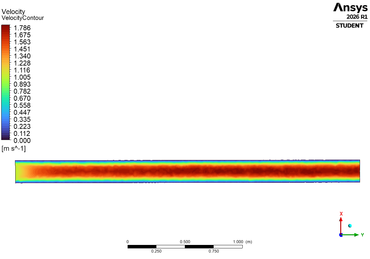
The contour makes the development region visible directly: the high-velocity core is narrower right at the inlet and widens over a short distance before the color band stabilizes for the rest of the pipe — a visual read on the flow becoming fully developed.

It's worth checking that number against theory. For fully-developed laminar pipe flow, the Hagen–Poiseuille solution predicts a parabolic profile with a centerline velocity of exactly twice the mean velocity:

v_max = 2 × v_avg = 2 × 1 m/s = 2.0 m/s

The simulated 1.79 m/s comes in about 10% under that fully-developed value. The hydrodynamic entrance length for this case, L_e ≈ 0.05·Re·D = 0.05(100)(0.2 m) = 1 m, says the profile should be essentially fully developed well before the 3 m outlet — so the gap is more likely attributable to the coarse default mesh and a modest 200-iteration run than to genuine entrance effects. A finer mesh and a tighter residual target would be the natural next step to close that gap.

Pressure Field Results

The same XY plane, now colored by static pressure instead of velocity, shows the field decreasing smoothly and monotonically from 101,330.82 Pa at the inlet to 101,325.00 Pa at the outlet. That outlet value lands almost exactly on the 101,325 Pa gauge pressure specified as the outlet boundary condition — the same setting discussed in the Design Decision above. The whole field sits in a narrow band clustered around atmospheric pressure, which is the point made there: the absolute level is just the outlet BC plus a near-constant offset, not a physically meaningful number on its own.

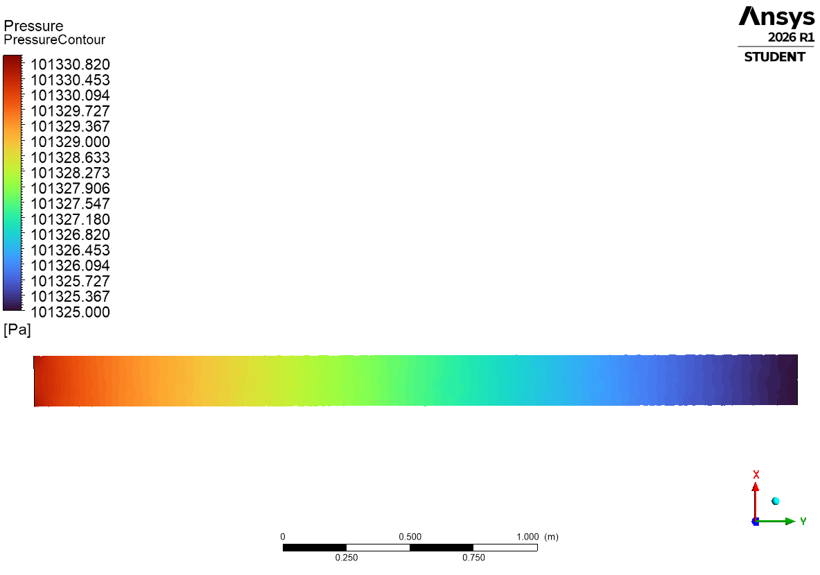
What is physically meaningful is the difference between those two numbers: a 5.82 Pa drop from inlet to outlet, which is the actual force per unit area pushing the fluid through the pipe against wall friction. Checked against the Hagen–Poiseuille friction-only prediction for fully-developed laminar flow:

ΔP = 32μLV / D² = 32(2×10^-3)(3)(1) / (0.2)² = 4.8 Pa

The simulated 5.82 Pa runs about 20% above that estimate. That's consistent with the same entrance-length story from the velocity results, not a contradiction of it: accelerating the flow from a flat inlet profile into its parabolic shape takes additional pressure drop beyond what pure fully-developed wall friction accounts for, so some premium over the friction-only number is exactly what should show up while part of the pipe is still developing.

Extended Post-Processing: Streamlines in Motion

Beyond the static contours, I used ANSYS CFD-Post's animation tool to trace streamline tracers advecting through the pipe, colored by local velocity magnitude — a technique adapted from a companion Fluent tutorial covering pipe-flow post-processing. It turns the same parabolic-profile result from a static color gradient into something you watch happen: tracers riding the centerline streamlines (orange-red, near the 1.79 m/s peak) visibly pull ahead of the tracers running close to the wall (green, moving at a fraction of that speed), to the point that the fastest, centermost tracers have already exited the pipe while the slowest, wall-adjacent ones are still only partway down its length. It's the same physics as the velocity contour and the profile discussion above — viscous shear at the wall dragging the flow to zero while the core rushes ahead — just made directly visible as motion instead of inferred from a color scale.

Key Takeaways